Alternatives to the Logistic Equation

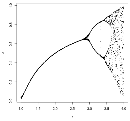Yesterday, I decided to plot the bifurcation diagram of the logistic equation.  This is a famous plot from the 70s, with which many geeks will be familiar.  It shows that simple systems can switch into "chaos mode" and begin to bifurcate wildly.

tl;dr: bifurcation.R

To produce the graphs, we use code in the R programming language.

First off, we set the range and maximum iterations for the plot:

# Set the range of the r values
r_range <- seq( 1, 4, 0.01 )

# Set the maximum number of x iterations
x_max <- 30

Next we initialize the vector to hold our points:

# Initialize the bucket of x's
v <- c()

Here are the guts of the program that collects the points to plot:

# For each r, find the x values...
for ( r in r_range ) {
    # Start at a low x value
    x <- 0.1
    # Repeat x_max times...
    for ( i in 0 : x_max ) {
        # The logistic equation
        x <- r * x * ( 1 - x )
        # Hopefully we have stabilized
        if ( i > x_max / 2 ) {
            v <- c( v, x )
        }
    }
}

The crucial bit, to keep in mind, is the line with the iterating logistic equation.

Lastly we plot the points and save the graph!

png(file = 'bifurcation.png')
plot(
    seq( 1, 4, length.out = length(v) ),
    v,
    type = 'p',
    cex  = 0.1,
    xlab = 'r',
    ylab = 'x'
)
dev.off()

OK.  Now that we have our traditional logistic equation bifurcation diagram, what can we do next?  How about finding other equations which produce bifurcation diagrams?  Check these out:

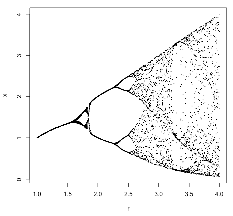
The equation, x <- r * x ** (1 - x) generates this plot:

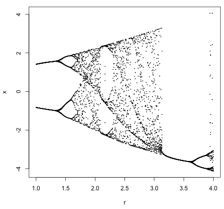
The equation, x <- r * cos(x) - sin(x) generates this plot:

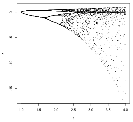
The equation, x <- r * exp(x) * (1 - exp(x)) generates this plot:

More alternative equations:

r - x ** 2  or  r ** cos(1 - x)  or  r * cos(x) * (1 - sin(x)) ...